What is Query, Key, and Value (QKV) in the Transformer Architecture and Why Are They Used?
An analysis of the intuition behind the notion of Key, Query, and Value in the Transformer architecture and why is it used.

TL;DR
QKV is used to mimic a “search” procedure, in order to find the pairwise similarity measures between tokens. Further, these similarity measures act as weights, to get a weighted average of tokens’ meanings, to make them contextualized.
Query acts as the part of a token’s meaning that is being searched, for similarity. Key acts as the part of all other tokens’ meanings that Query is compared against. This comparison is done by the dot-product of their vectors which results in the pairwise similarity measures, which is then turned into pairwise weights by normalizing (i.e. Softmax). Value is the part of a token’s meaning that is combined in the end using the found weights.
Lastly, you might have noticed me saying each of QKV being “part of a token’s meaning”. By that, I mean each of the QKV is obtained by a learned transformation of a token’s initial embedding. Hence, each can be learned to extract a specific different meaning from the embedding. And by employing, Multi-head attention, we allow multiple different contexts being propagated through the network.
Introduction
Recent years have seen the Transformer architecture make waves in the field of natural language processing (NLP), achieving state-of-the-art results in a variety of tasks including machine translation, language modeling, and text summarization, as well as other domains of AI i.e. Vision, Speech, RL, etc.
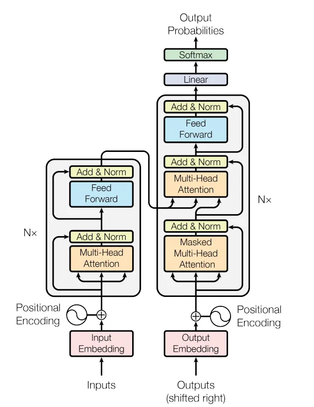
Vaswani et al. (2017), first introduced the transformer in their paper “Attention Is All You Need”, in which they used the self-attention mechanism without incorporating recurrent connections while the model can focus selectively on specific portions of input sequences.
In particular, previous sequence models, such as recurrent encoder-decoder models, were limited in their ability to capture long-term dependencies and parallel computations. In fact, right before the Transformers paper came out in 2017, state-of-the-art performance in most NLP tasks was obtained by using RNNs with an attention mechanism on top, so attention kind of existed before transformers. By introducing the multi-head attention mechanism on its own, and dropping the RNN part, the transformer architecture resolves these issues by allowing multiple independent attention mechanisms.
In this post, we will go over one of the details of this architecture, namely the Query, Key, and Values, and try to make sense of the intuition used behind this part.
Note that this post assumes you are already familiar with some basic concepts in NLP and deep learning such as embeddings, Linear (dense) layers, and in general how a simple neural network works.
Attention!
First, let’s start understanding what the attention mechanism is trying to achieve. And for the sake of simplicity, let’s start with a simple case of sequential data to understand what problem exactly we are going to solve, without going through all the jargon of the attention mechanism.
Context Matters
Consider the case of smoothing time-series data. Time series are known to be one of the most basic kinds of sequential data due to the fact that it is already in a numerical and structured form, and is usually in low-dimensional space. So it would be suitable to lay out a good starting example.
To smooth a highly variant time series, a common technique is to calculate a “weighted average” of the proximate timesteps for each timestep, as shown in image 1, the weights are usually chosen based on how close the proximate timesteps are to our desired timestep. For instance, in Gaussian Smoothing, these weights are drawn from a Gaussian function that is centered at our current step.

What we have done here, in a sense, is that:
-
We took a sequence of values,
-
And for each step of this sequence, we added (a weighted) context from its proximate values, while the proportion of added context (the weight) is only related to their proximity to the target value.
-
And finally, we attained a new contextualized sequence, which we can understand and analyze more easily.
There are two key points/issues in this example:
-
It only uses the proximity and ordinal position of the values to obtain the weights of the context.
-
The weights are calculated by fixed arbitrary rules for all points.
The Case of Language
In machine learning, textual data always have to be represented by vectors of real-valued numbers AKA Embeddings. So we assume that the primary meanings of tokens (or words) are encoded in these vectors. Now in the case of textual sequence data, if we would like to apply the same kind of technique to contextualize each token of the sequence as the above example so that each token’s new embedding would contain more information about its context, we would encounter some issues which we will discuss now:
Firstly, in the example above, we only used the proximity of tokens to determine the importance (weights) of the context to be added, while words do not work like that. In language, the context of a word in a sentence is not based only on the ordinal distance and proximity. We can’t just blindly use proximity to incorporate context from other words.
Secondly, adding the context only by taking the (weighted) average of the embeddings of the context tokens itself may not be entirely intuitive. A token’s embedding may contain information about different syntactical, semantical, or lexical aspects of that token. All of this information may not be relevant to the target token to be added. So it’s better not to add all the information as a whole as context.
So if we have some (vector) representation of words in a sequence, how do we obtain the weights and the relevant context to re-weight and contextualize each token of the sequence?
The answer, in a broad sense, is that we have to “search” for it, based on some specific aspects of the tokens meaning (could be semantic, syntactic, or anything). And during this search, assign the weights and the context information based on relevance or importance.
It means that for each of the tokens in a sequence, we have to go through all other tokens in the sequence, and assign them weights and the context information, based on a similarity metric that we use to compare our target token with others. The more similar they are in terms of the desired context, the larger the weight it gets.
So, in general, we could say that the attention mechanism is basically (1) assigning weights to and (2) extracting relevant context from other tokens of a sequence based on their relevance or importance to a target token (i.e. attending to them).
And we said that in order to find this relevance/importance we need to search through our sequence and compare tokens one-to-one.

This is where the Query, Key, and Values find meaning.
Query, Key, and Value
To make more sense, think of when you search for something on YouTube, for example. Assume YouTube stores all its videos as a pair of “video title” and the “video file” itself. Which we call a Key-Value pair, with the Key being the video title and the Value being the video itself.
The text you put in the search box is called a Query in search terms. So in a sense, when you search for something, YouTube compares your search Query with the Keys of all its videos, then measures the similarity between them, and ranks their Values from the highest similarity down.

In our problem, we have a sequence of token vectors, and we want to search for the weights to re-weight and contextualize each token (word) embedding of the sequence, we can think in terms of:
-
What you want to look for is the Query.
-
What you are searching among is Key-Value pairs.
-
The query is compared to all the Keys to measure the relevance/importance/similarity.
-
The Values are utilized based on the assigned similarity measure.
Another helpful relevant analogy is a dictionary (or hashmap) data structure. A dictionary stores data in key-value pairs and it maps keys to their respective value pairs. When you try to get a specific value from the dictionary, you have to provide a query to match its corresponding key, then it searches among those keys, compares them with the query, and if matched, the desired value will be returned.
However, the difference here is that this is a “hard-matching” case, where the Query either exactly matches the Key or it doesn’t and an in-between similarity is not measured between them.

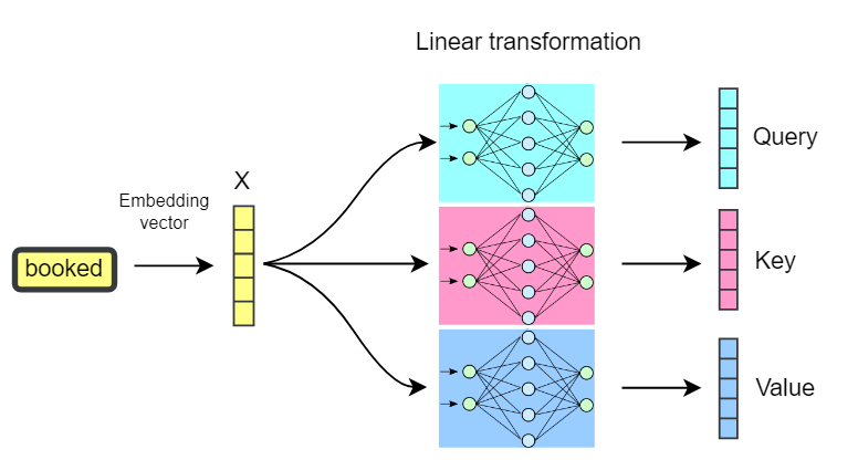
We earlier mentioned that we are only working with real-valued vectors (token embeddings). So the Query, Key, and Value also need to be vectors. However, so far we only have one vector for each token which is its embedding vector. So, how should we obtain the Query, Key, and Value vectors?
We Construct them using linear projections (linear transformations aka single dense layer with separate sets of weights: Wq, Wₖ, Wᵥ) of the embedding vector of each token. This means we use a learnable vector of weights for each of the Query, Key, and Value to do a linear transformation on the word embedding to obtain the corresponding Query, Key, and Value vectors.
An embedding of a token may represent different contextual, structural, and syntactical aspects of that token. By using learnable linear transformation layers to construct these vectors from the token’s embedding, we allow the network to:
-
Extract and pass a limited specific part of that information into the Q, K, and V vectors.
-
Determine a narrower context in which the search and match is going to be done.
-
Learn what information in an embedding is more important to attend to.
Now, having the Q, K, and V vectors in hand, we are able to perform the “search and compare” procedure that was discussed before, with these vectors. This results in the final derivation of the attention mechanism proposed in the proposed in (Vaswani et al 2017).
For each token:
-
We compare its Query vector to all other tokens’ Key vectors.
-
Calculate a vector similarity score between each two (i.e. the dot-product similarity in the original paper)
-
Transform these similarity scores into weights by scaling them into [0,1] (i.e. Softmax)
-
And add the weighted context by weighting their corresponding value vectors.

So the whole notion of the Q, K, and V vectors is like a soft dictionary to mimic a search-and-match procedure from which we learn how much two tokens in a sequence are relevant (the weights), and what should be added as the context (the values). Also, note that this process does not have to happen sequentially (one token at a time). This all happens in parallel by using matrix operations.
Note that in the illustration below, the matrix dimensions are switched compared to that of the original paper (n_tokens by dim instead of dim by n_tokens). Later in this post, you will see the original and complete formulation of the attention mechanism which is the other way around.
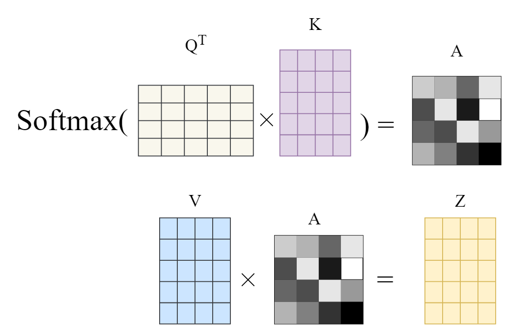
This results in a more context-aware embedding of each token, where the added context is based on the relevance of the tokens to each other and it is learned through Q, K, V vector transformation. Hence, the dot-product attention mechanism. The original attention mechanism in (Vaswani et al, 2017) also scales the dot-product of K and Q vectors, meaning it divides the resulting vector by sqrt(d), where d is the dimension of the Query vector. Hence the name, “scaled dot-product attention”. This scaling helps with reducing the variance of the dot-product before being passed to the Softmax function:

Finally, we mentioned that the linear layers that transform the embedding into Q, K, V, may extract only a specific pattern in the embedding for finding the attention weights. To enable the model to learn different complex relations between the sequence tokens, create and use multiple different versions of these Q, K, V, so that each will focus on different patterns existing in our embeddings. These multiple versions are called attention heads resulting in the name “multi-head attention”. These heads can also be vectorized and computed in parallel using current popular deep learning frameworks.

Conclusion
So to wrap up, in this post I tried to picture and analyze the intuition behind the use of Query, Key, and Value which are key components in the attention mechanism and may be a little difficult to make sense of, at first encounters.
The attention mechanism discussed in this post was proposed in the transformer architecture that is introduced in the (Vaswani et al, 2017) paper “Attention is all you need” and has been one of the top-performing architectures since, in several different tasks and benchmarks in deep learning. With its vast use cases and applicability, it would be helpful to have an understanding of the intuition behind the nuts and bolts used in this architecture and know why we use it.
I attempted to be as clear and as basic as possible while explaining this topic by laying down examples and illustrations wherever possible.
References
[1] Vaswani, Ashish, Noam Shazeer, Niki Parmar, Jakob Uszkoreit, Llion Jones, Aidan N. Gomez, Lukasz Kaiser, and Illia Polosukhin. “Attention Is All You Need.” arXiv, August 1, 2023. https://doi.org/10.48550/arXiv.1706.03762.