Solve Optimization Problems on Google Cloud Platform using Google’s OR API and OR-tools MathOpt
A quick guide to implementing and solving mathematical optimization models using Google Cloud Platform (GCP) with OR-tools MathOpt interface and OR API endpoints in Python.
A quick guide to implementing and solving mathematical optimization models using Google Cloud Platform (GCP) with OR-tools MathOpt interface and OR API endpoints in Python.

Introduction
Operations Research and Mathematical Optimization practitioners and developers often face challenges when dealing with large-scale or even medium-sized optimization problems on their local machines, such as hardware and resource constraints, dependency management, etc.
Google’s new OR API, part of the OR-tools suite, offers a solution by allowing users to solve linear, mixed-integer, and quadratic programming problems on remote cloud services of GCP. This way we can use Google’s computing infrastructure to handle solving complex models that might be impractical to solve on a single machine due to memory or time constraints.

In this post, we’ll explore how to use this API to formulate and solve optimization problems, focusing on its integration with OR-Tools, Google’s open-source software suite for optimization. We’ll cover the basics of problem formulation, discuss the supported solvers like GLOP, PDLP, and SCIP, and walk through the process of sending models to the cloud service for resolution.
Supported Problems
Google’s OR API offers two problem-specific endpoints as well as a general endpoint to solve any custom modeled mathematical program.
The problem-specific endpoints will not be the main focus of this post. Feel free to dig into their documentation if the suit your needs. These endpoints cover:
-
Workforce Scheduling: offers two solvers using the SolveShiftGeneration and SolveShiftScheduling methods.
-
Shipping Network Design:Solves the Liner Shipping Network Design and Scheduling Problem (LSNDSP). The problem involves the design and scheduling of a liner shipping network that minimizes operational costs, while maximizing revenue from the shipping of commodity demand between ports.
The general endpoint, namely The MathOpt Service, uses MathOpt as input format. MathOpt is a new feature from the Google OR-tools suite that provides a unified modelling interface, that separates modelling and solving stages in math programming. After modelling is done in MathOpt, the model can be coupled up with any different Solvers and methods by just easily changing an ENUM for the solver parameter, for faster and better experiments. We’ll see how it’s done below in examples.
In terms of generality, MathOpt models can contain:
-
Integer or continuous variables
-
Linear or quadratic constraints
-
Linear or quadratic objectives
Models are defined independently of any solver and solvers can be swapped interchangeably. Currently following solvers are supported in MathOpt Service (the cloud endpoint):
-
GLOP: Google’s Glop linear solver. Supports LP with primal and dual simplex methods.
-
PDLP: Google’s PDLP solver. Supports LP and convex diagonal quadratic objectives. Uses first order methods rather than simplex. Can solve very large problems.
-
CP-SAT: Google’s CP-SAT solver. Supports problems where all variables are integer and bounded (or implied to be after presolve).
-
SCIP: Solving Constraint Integer Programs (SCIP) solver (third party). Supports LP, MIP, and nonconvex integer quadratic problems. No dual data for LPs is returned though. Prefer GLOP for LPs.
-
GLPK: GNU Linear Programming Kit (GLPK) (third party). Supports MIP and LP.
-
OSQP: The Operator Splitting Quadratic Program (OSQP) solver (third party). Supports continuous problems with linear constraints and linear or convex quadratic objectives. Uses a first-order method.
-
HiGHS: The HiGHS Solver (third party). Supports LP and MIP problems (convex QPs are unimplemented).
Note that MathOpt itself supports a wider range of solver, the above were the one currently supported in the OR API.
How to use it + Examples
In general, the process of solving a model using MathOpt Service has three steps:
-
Modelling
-
Solver Parameter Setting
-
Making a request to OR API.
But first, you have to follow THESE INITIAL STEPS once, to obtain your OR api_key from GCP. You also need to have OR-tools installed locally. See how to install OR-tools.
Step 1: Modelling
All the modelling is done through the mathopt module. In python, it is imported as follows:
from ortools.math_opt.python import mathopt
Example 1:
Consider the following Linear Program (LP):
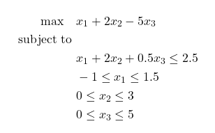
Then modelling using the mathopt interface is as easy as:
# Example 1: Simple LP
model = mathopt.Model(name="example_lp")
x_1 = model.add_variable(lb=-1., ub=1.5, is_integer=False, name="x_1")
x_2 = model.add_variable(lb= 0., ub=3. , is_integer=False, name="x_2")
x_3 = model.add_variable(lb= 0., ub=5. , is_integer=False, name="x_3")
model.add_linear_constraint(x_1 + 2*x_2 + 0.5*x_3 <= 2.5)
model.maximize(x_1 + 2*x_2 - 5*x_3)
Example 2:
Consider a basic N by N assignment problem with the following integer (binary) linear program:

where decision variable x_ij is 1 if source i is assigned to target j, and 0 otherwise. And the constraints make sure each source is exactly assigned to one target and vice versa. This model is implemented using mathopt as follows:
# Example 1: Assignment IP

# n: number of sources/targets
# W: nxn numpy array of coefficients

model = mathopt.Model(name="example_assignment")
X_mat = [
            [model.add_binary_variable(name=f"x_{i}_{j}") for j in range(n)]
            for i in range(n)
            # equivalently can use either:
            # model.add_variable(lb=0., ub=1., is_integer=True, name=f"x_{i}_{j}")
            # model.add_integer_variable(lb=0., ub=1., name=f"x_{i}_{j}")
      ]

# Objective function
obj = sum(
      W[s][t] * X_mat[s][t]
      for s in range(n) # source indices
      for t in range(n) # target indices
      )
# Consraintsfunction
for i in range(n):
      model.add_linear_constraint(sum(X_mat[i][j] for j in range(n)) == 1)
      model.add_linear_constraint(sum(X_mat[j][i] for j in range(n)) == 1)
That all! Now let’s see how we can solve these models.
Steps 2–3: Parameter Setting and Solving
In general when we not use the GCP API service, and want to solve a model such as the above mentioned example models locally with mathopt. The models are solved as follows:
    params = mathopt.SolveParameters(enable_output=True)
    result = mathopt.solve(model, mathopt.SolverType.GLOP, params=params)
    if result.termination.reason != mathopt.TerminationReason.OPTIMAL:
        raise RuntimeError(f"model failed to solve: {result.termination}")
As you can see, it does not really matter which model (from example 1 or 2) we want to solve, the process is the same nonetheless. The important point is to select the most appropriate solver for our problem. The solver can be changed using the corresponding ENUM from the following list:
# Solvers supported in MathOpt Service (OR API)
GSCIP:     mathopt.SolverType.GSCIP
GLOP:      mathopt.SolverType.GLOP
CP_SAT:    mathopt.SolverType.CP_SAT
PDLP:      mathopt.SolverType.PDLP
GLPK:      mathopt.SolverType.GLPK
OSQP:      mathopt.SolverType.OSQP
HIGHS:     mathopt.SolverType.HIGHS

# Additional sovers for local use
ECOS:      mathopt.SolverType.ECOS
SCS:       mathopt.SolverType.SCS
GUROBI:    mathopt.SolverType.GUROBI
SANTORINI: mathopt.SolverType.SANTORINI
For parameters argument params you are able to set the following additional parameters depending on the chosen solver:
- time_limit: The maximum time a solver should spend on the problem,
- iteration_limit: Limit on the iterations of the underlying algorithm (e.g.
      simplex pivots).
- node_limit: Limit on the number of subproblems solved in enumerative search
      (e.g. branch and bound).
- cutoff_limit: The solver stops early if it can prove there are no primal
      solutions at least as good as cutoff.
- objective_limit: The solver stops early as soon as it finds a solution at
      least this good, with TerminationReason.FEASIBLE and Limit.OBJECTIVE.
- best_bound_limit: The solver stops early as soon as it proves the best bound
      is at least this good, with TerminationReason of FEASIBLE or
      NO_SOLUTION_FOUND and Limit.OBJECTIVE.
- solution_limit: The solver stops early after finding this many feasible
      solutions, with TerminationReason.FEASIBLE and Limit.SOLUTION. Must be
      greater than zero if set
- enable_output: If the solver should print out its log messages.
- absolute_gap_tolerance: An absolute optimality tolerance (primarily) for MIP
      solvers. The absolute GAP is the absolute value of the difference between

- relative_gap_tolerance: A relative optimality tolerance (primarily) for MIP
      solvers. The relative GAP is a normalized version of the absolute GAP.
- solution_pool_size: Maintain up to `solution_pool_size` solutions while
      searching.
- lp_algorithm: The algorithm for solving a linear program. If UNSPECIFIED,
      use the solver default algorithm.
- presolve: Effort on simplifying the problem before starting the main
      algorithm (e.g. simplex).
- cuts: Effort on getting a stronger LP relaxation (MIP only). Note that in
      some solvers, disabling cuts may prevent callbacks from having a chance to
      add cuts at MIP_NODE.
- heuristics: Effort in finding feasible solutions beyond those encountered in
      the complete search procedure.
- scaling: Effort in rescaling the problem to improve numerical stability.
- gscip: GSCIP specific solve parameters.
- gurobi: Gurobi specific solve parameters.
- glop: Glop specific solve parameters.
- cp_sat: CP-SAT specific solve parameters.
- pdlp: PDLP specific solve parameters.
- osqp: OSQP specific solve parameters.
- glpk: GLPK specific solve parameters.
- highs: HiGHS specific solve parameters.
You can check out MathOpt’s source code here for more details on supporting parameters.
Now when using the OR API to solve the model remotely on GCP, the procedure differs a little bit. For this, we use the remote_http_solve module from OR-tools, as follows:
from ortools.math_opt.python import mathopt
from ortools.math_opt.python.ipc import remote_http_solve

# Read the API Key from a JSON file with the format:
# {"key": "your_api_key"}
with open("credentials.json") as f:
      credentials = json.load(f)
      api_key = credentials["key"]

model = ... # define the model similar to examples 1,2 above

try:
      # solving remotely on GCP
      result, logs = remote_http_solve.remote_http_solve(
      model,
      mathopt.SolverType.GSCIP,   # or any solver from the list above
      mathopt.SolveParameters(enable_output=True),
      api_key=api_key, # Other additional solving parameters can be set from the above list
      )
      sol_obj = result.objective_value()
      sol_var = result.variable_values()
      sol_var = {var.name: val for var, val in sol_var.items()}


      print("Objective value: ", sol_obj)
      print("Solution: ", sol_var)
      print("\n".join(logs))

except remote_http_solve.OptimizationServiceError as err:
      print(err)
That’s it! You solved a model without depending on your machine’s resources completely remotely on GCP.
See the complete code examples below:
Example 1:
Example 2: (Assignment problem ILP)
For more information about Google OR-tools’ new MathOpt module you can also check these resources out: