First-order methods in Linear Programming: PDHG and GPU-friendly LP solvers
An introduction to first-order methods for linear programming, focusing on the Primal-Dual Hybrid Gradient (PDHG), the algorithm behind GPU-accelerated LP solvers, and its practical enhancements.
Introduction: The GPU Era in Constrained Optimization
If you’ve been following the optimization community lately, you might have noticed something interesting happening: GPUs are finally coming for linear programming.
For decades, linear programming (LP) solvers have been dominated by two workhorses: the simplex method and interior-point methods (IPMs). These methods are mature, reliable, and backed by decades of theoretical and practical refinement. But they have a challenge: as problems grow to massive scale, their reliance on matrix factorizations and sequential operations becomes a bottleneck, especially on modern parallel hardware like GPUs.
The New Wave of GPU-Accelerated Solvers
In the past couple of years, we’ve seen an explosion of interest in GPU-accelerated LP solvers:
-
NVIDIA cuOpt (2024): NVIDIA released and open-sourced cuOpt, a GPU-accelerated optimization engine that excels in mixed integer linear programming (MILP), linear programming (LP), and vehicle routing problems (VRP). Their developer blog demonstrates substantial speedups on large-scale problems.
-
Gurobi Integration: The industry-leading commercial solver Gurobi adopted GPU acceleration based on similar first-order methods, recognizing the potential of this approach.
-
Open-Source Ecosystem: A vibrant ecosystem of open-source solvers emerged, including cuPDLPx and cuPDLP.jl, Google’s PDLP, and MPAX.
But here’s the interesting part: all of these solvers are built on first-order methods (FOMs), specifically variants of the Primal-Dual Hybrid Gradient (PDHG) algorithm. This represents a different philosophy from traditional LP solving, and it’s worth understanding why this approach is gaining traction.
Why First-Order Methods? Why GPUs?
The key insight is simple: GPUs excel at massively parallel operations, particularly matrix-vector multiplications. Modern GPUs can perform thousands of such operations simultaneously with enormous throughput. Traditional LP methods (simplex and IPMs) rely heavily on solving linear systems via matrix factorizations—operations that are inherently sequential and difficult to parallelize effectively.
First-order methods, on the other hand, are built around simple iterative updates involving matrix-vector products: $Ax$, $A^Ty$. No factorizations. No solving linear systems. Just multiply and update. This computational profile aligns beautifully with GPU architectures.
The tradeoff? First-order methods typically require more iterations to converge than their second-order counterparts. But when each iteration can be dramatically faster on a GPU, this iteration count penalty often becomes irrelevant—especially for massive problems where factorization costs grow prohibitively.
Building PDHG from Scratch: A Walk Through First-Order Methods for LP
Let’s understand how we arrived at PDHG by starting from scratch. We’ll attempt to build a first-order method for LP, see where each approach fails, and understand how PDHG elegantly resolves these challenges.
The Linear Programming Problem
Consider the standard form LP:
\[\begin{align} \min_{x \in \mathbb{R}^n} \quad & c^T x \\ \text{s.t.} \quad & Ax = b \\ & x \geq 0 \end{align}\]where \(A \in \mathbb{R}^{m \times n}\), \(b \in \mathbb{R}^m\), and \(c \in \mathbb{R}^n\). The dual problem is:
\[\begin{align} \max_{y \in \mathbb{R}^m} \quad & b^T y \\ \text{s.t.} \quad & A^T y \leq c \end{align}\]Our goal is to find a first-order method that:
- Uses only simple operations (especially matrix-vector products)
- Avoids solving linear systems or factorizations
- Actually converges to an optimal solution
- Can leverage parallel hardware like GPUs
1. Projected Gradient Descent (PGD)
Why start here? For unconstrained optimization, gradient descent is the canonical first-order method. When we have constraints, the natural extension is projected gradient descent: take a gradient step, then project back onto the feasible set.
The algorithm would be:
\[x^{k+1} = \text{proj}_{\mathcal{C}}(x^k - \eta c)\]where \(\mathcal{C} = \{x \in \mathbb{R}^n : Ax = b, x \geq 0\}\) is our feasible set and \(\eta > 0\) is the step-size.
What is projection? The projection of a point \(z\) onto a set \(\mathcal{C}\) is the closest point in \(\mathcal{C}\) to \(z\):
\[\text{proj}_{\mathcal{C}}(z) = \arg\min_{x \in \mathcal{C}} \|x - z\|^2\]Geometrically, it’s like “snapping” \(z\) to the nearest feasible point.
How is it computed? This depends on the set \(\mathcal{C}\):
- For simple sets like boxes ($l \leq x \leq u$), projection is trivial: just clamp each coordinate
- For our LP constraints \(\{x : Ax = b, x \geq 0\}\), projection requires solving:
This is itself a quadratic program with equality and inequality constraints!
The Problem: Solving this QP requires:
- Either forming and solving a linear system \(A(A^T)^{-1}\) (if we eliminate the equality constraints)
- Or using an iterative QP solver
Both options involve solving linear systems or running an optimization algorithm inside our optimization algorithm. For large-scale LP, computing the projection can be as expensive as solving the original problem! This defeats our goal of having a simple, GPU-friendly method.
Key Insight: We need to somehow handle the constraints separately—keeping the “easy” constraints (like \(x \geq 0\)) and dealing with the “hard” constraints (like \(Ax = b\)) differently.
2. Dualization and Gradient Descent-Ascent (GDA)
Why move to a primal-dual approach? The key observation is that our constraints fall into two categories:
- Simple constraints: \(x \geq 0\) (projection is trivial: \(\max(x, 0)\) element-wise)
- Complex constraints: \(Ax = b\) (projection requires solving a system)
What if we could keep the simple constraints explicit and handle the complex ones differently?
The solution: Use Lagrangian duality. Instead of projecting onto \(Ax = b\), we dualize this constraint by introducing dual variables \(y\) and work with the Lagrangian:
\[\mathcal{L}(x, y) = c^T x + y^T(b - Ax)\]Notice that:
- If \(Ax = b\) (primal feasible), then \(y^T(b - Ax) = 0\) and \(\mathcal{L}(x,y) = c^T x\)
- If \(Ax \neq b\), we can pick \(y\) to make \(\mathcal{L}(x,y)\) arbitrarily bad
This gives us the primal-dual formulation:
\[\min_{x \geq 0} \max_{y} \mathcal{L}(x, y) = \min_{x \geq 0} \max_{y} \left[ c^T x - y^T Ax + b^T y \right]\]More compactly, with the indicator function \(\iota_{\mathbb{R}^n_+}(x)\) (which is 0 if \(x \geq 0\), infinity otherwise):
\[\min_{x} \max_{y} L(x, y) := c^T x + \iota_{\mathbb{R}^n_+}(x) - y^T A x + b^T y\]Why is this better?
- By convex duality theory, saddle points \((x^*, y^*)\) of this Lagrangian correspond to optimal primal-dual pairs
- Now we only need to project onto \(x \geq 0\), which is trivial!
- We’ve traded one hard projection for a saddle point problem
Gradient Descent-Ascent: For saddle point problems, the natural first-order method is gradient descent in \(x\) (minimization) and gradient ascent in \(y\) (maximization):
\[\begin{align} x^{k+1} &= \text{proj}_{\mathbb{R}^n_+}(x^k - \eta \nabla_x L(x^k, y^k)) \\ &= \text{proj}_{\mathbb{R}^n_+}(x^k - \eta(c - A^T y^k)) \\ &= \max(x^k + \eta A^T y^k - \eta c, 0) \\[1em] y^{k+1} &= y^k + \sigma \nabla_y L(x^k, y^k) \\ &= y^k + \sigma(b - A x^k) \\ &= y^k - \sigma A x^k + \sigma b \end{align}\]where \(\eta, \sigma > 0\) are primal and dual step-sizes. The projection is now just a max operation—exactly what we wanted!
Does it work? Let’s test on a simple example.
Consider the simple bilinear saddle point problem:
\[\min_{x \geq 0} \max_y (x - 3)y\]The unique saddle point is at \((x^*, y^*) = (3, 0)\). Starting from \((x^0, y^0) = (2, 2)\) with step-sizes \(\eta = \sigma = 0.2\), GDA gives:
# Simple GDA example showing divergence
def gda_update(x, y, eta=0.2, sigma=0.2):
    x_new = max(0, x - eta * y)      # gradient of L w.r.t. x is y
    y_new = y + sigma * (3 - x)      # gradient of L w.r.t. y is (x - 3)
    return x_new, y_new

# Run GDA from (2, 2)
x, y = 2.0, 2.0
for iteration in range(50):
    x, y = gda_update(x, y)
    if x > 10 or abs(y) > 10:  # Diverging!
        print(f"Diverged at iteration {iteration}")
        break

# Output: Diverged at iteration 15
The iterates spiral outward rather than converging to \((3, 0)\). Plotting the trajectory shows ever-widening circles.
Why does GDA fail? The problem is that GDA updates each variable based on the gradient at the current point. For saddle point problems, this creates a “chasing” behavior where \(x\) and \(y\) oscillate and amplify each other’s errors rather than correcting them. Mathematically, the update matrix has eigenvalues outside the unit circle, causing divergence.
This is a fundamental limitation: GDA does not converge for bilinear saddle point problems (which includes all LPs!). We need something better.
3. Proximal Point Method (PPM)
Why does GDA fail, and what fixes it? GDA fails because it uses gradient information from the current iterate, creating instability. What if we could use gradient information from the next iterate instead?
This is the idea behind the Proximal Point Method. Instead of the explicit update: \(x^{k+1} = x^k - \eta \nabla f(x^k)\)
PPM solves an implicit equation: \(x^{k+1} = x^k - \eta \nabla f(x^{k+1})\)
For our saddle point problem, this becomes:
\[(x^{k+1}, y^{k+1}) = \arg\min_{x \geq 0} \max_y \left[ L(x, y) + \frac{1}{2\eta}\|x - x^k\|^2 - \frac{1}{2\sigma}\|y - y^k\|^2 \right]\]The quadratic penalty terms \(\frac{1}{2\eta}\|x - x^k\|^2\) and \(-\frac{1}{2\sigma}\|y - y^k\|^2\) act as regularizers, preventing the iterates from moving too far in one step.
Why this works: The implicit gradient creates a stabilizing effect. Geometrically, we’re not just following the gradient direction blindly—we’re finding a point that balances between:
- Moving in the gradient direction (improving the objective)
- Staying close to the current iterate (stability)
This regularization fixes GDA’s divergence problem. In fact, on the same toy problem where GDA diverged, PPM would converge smoothly to the saddle point!
The catch: This is an implicit update. To compute \((x^{k+1}, y^{k+1})\), we need to solve the saddle point problem shown above at every iteration. This subproblem is nearly as expensive as our original LP for large-scale problems—completely impractical.
The dilemma:
- GDA is explicit and cheap per iteration, but diverges
- PPM converges beautifully, but requires solving a subproblem at each step
Can we get the best of both worlds?
The Solution: Primal-Dual Hybrid Gradient (PDHG)
Yes! PDHG (also known as the Chambolle-Pock algorithm, after its originators) ingeniously combines explicit computation with convergence guarantees.
The key insight: What if we could approximate the implicit PPM update without actually solving it? PDHG achieves this through an extrapolation trick:
\[\begin{align} x^{k+1} &\leftarrow \text{proj}_{\mathbb{R}^n_+}(x^k + \eta A^T y^k - \eta c) \quad \text{(primal update, like GDA)} \\ y^{k+1} &\leftarrow y^k - \sigma A(\textcolor{red}{2x^{k+1} - x^k}) + \sigma b \quad \text{(dual update with extrapolation!)} \end{align}\]The primal update is identical to GDA. The magic is in the dual update: instead of using \(x^k\) or \(x^{k+1}\), we use \(\textcolor{red}{2x^{k+1} - x^k}\).
What is this extrapolated point?
Let’s break down \(2x^{k+1} - x^k\): \(2x^{k+1} - x^k = x^{k+1} + \underbrace{(x^{k+1} - x^k)}_{\text{displacement}}\)
This is the current iterate plus the displacement vector. Geometrically, it’s extrapolating along the direction of movement, predicting where the primal variable is “heading.”
Why does the extrapolation work?
Think about what we’re trying to fix from GDA. In GDA, the dual update at iteration \(k\) uses \(x^k\), which is “stale”—by the time we compute \(y^{k+1}\), we already have the newer \(x^{k+1}\). Using \(x^{k+1}\) directly would be better, but still not ideal.
The extrapolation \(2x^{k+1} - x^k\) goes further: it estimates what \(x^{k+2}\) might be. This implicitly approximates the “next iterate” idea from PPM, but without solving the implicit problem!
Multiple theoretical perspectives:
-
Operator theory: PDHG can be proven equivalent to a preconditioned proximal point method, inheriting PPM’s convergence guarantees
-
Predictor-corrector: The primal step predicts the next \(x\); the extrapolation corrects for this prediction in the dual update
-
Momentum interpretation: Rewriting as \(x^{k+1} + (x^{k+1} - x^k)\) shows it adds momentum to the iterate
Let’s verify this actually works on our toy problem:
def pdhg_update(x, y, eta=0.2, sigma=0.2):
    x_new = max(0, x - eta * y)
    y_new = y + sigma * (2*x_new - x - 3)  # Extrapolation!
    return x_new, y_new

# Run PDHG from same starting point (2, 2) where GDA diverged
x, y = 2.0, 2.0
for iteration in range(100):
    x, y = pdhg_update(x, y)
    if iteration % 20 == 0:
        print(f"Iteration {iteration}: x = {x:.4f}, y = {y:.4f}")

# Result: Converges to (3.0, 0.0)!
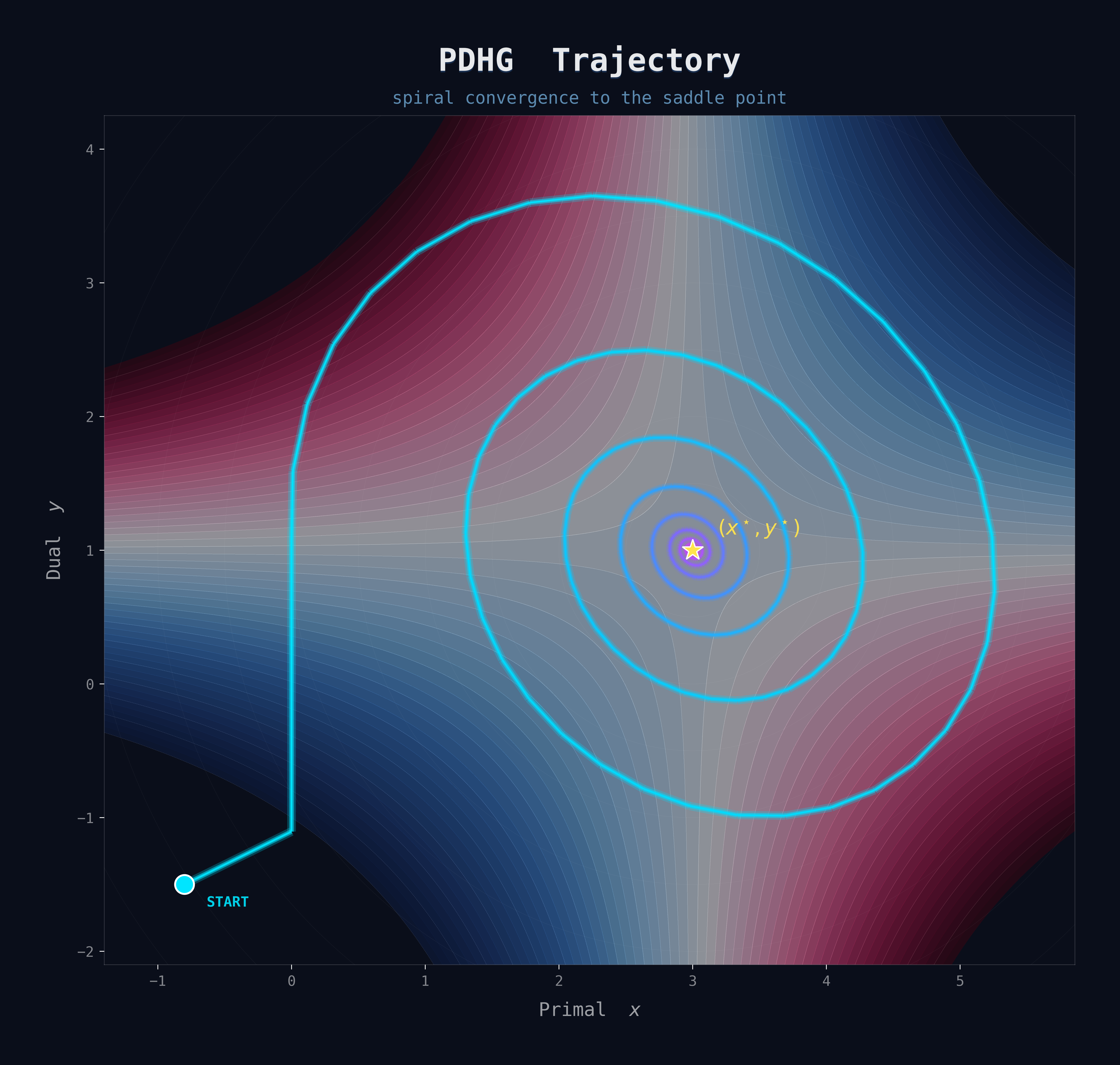
It works! With PDHG, the iterates spiral inward toward the saddle point \((3, 0)\). The extrapolation provides just enough stabilization to ensure convergence, giving us:
- Explicit, simple iterations (like GDA)
- Guaranteed convergence (like PPM)
- No subproblems to solve (unlike PPM)
This is exactly what we needed!
The Computational Advantage
Now we see why PDHG is perfect for GPU-accelerated LP solving. Each PDHG iteration requires only:
- Two matrix-vector products: \(A^T y\) and \(A(2x^{k+1} - x^k)\)
- Element-wise operations: Additions, subtractions, and max operations for projection
That’s it! No linear system solves. No matrix factorizations. No iterative subsolvers. Everything is:
- Explicit: Each operation has a closed-form expression
- Parallelizable: Matrix-vector products and element-wise ops parallelize perfectly
- Memory-efficient: Only need to store \(x\), \(y\), and the matrix \(A\)
This computational profile is perfectly suited for GPUs, which excel at:
- Massively parallel matrix-vector multiplications
- Simple arithmetic operations across large vectors
- Operations that don’t require sequential dependencies
Summary so far:
- PGD: Projection too expensive (requires solving a QP)
- GDA: Simple and cheap, but diverges
- PPM: Converges, but requires solving a subproblem
- PDHG: Explicit, converges, and GPU-friendly!
The Spiral Dynamics of PDHG
One fascinating observed property of PDHG when applied to LP is its distinctive spiral ray behavior. When visualizing the trajectory of iterates in primal-dual space, you often see a spiral pattern.
Within phases where the active set of variables (which variables are at their bounds) remains constant, the behavior can be understood through a dynamical systems lens. The iterates exhibit two simultaneous behaviors:
- Spiral-in rotation: The iterates circle toward a central point, improving primal and dual feasibility
- Forward movement: The iterates progress along a ray direction, improving the optimality gap
When the active set changes—when a variable hits its bound or leaves it—the algorithm transitions to a new spiral pattern with a different center and ray direction. This phase-by-phase behavior is characteristic of first-order primal-dual algorithms on LP and differs fundamentally from the edge-following behavior of simplex methods or the central-path-following behavior of interior-point methods.
PDLP: Making PDHG Production-Ready
While vanilla PDHG is elegant, it’s not ready for prime time. To build a practical, general-purpose LP solver, we need several enhancements. This is where PDLP (Primal-Dual hybrid gradient for Linear Programming) comes in.
The General LP Form
PDLP works with a more general LP formulation than the standard form:
\[\begin{align} \min_x \quad & c^T x \\ \text{s.t.} \quad & Ax = b \\ & Gx \geq h \\ & l \leq x \leq u \end{align}\]where \(G \in \mathbb{R}^{m_1 \times n}\), \(A \in \mathbb{R}^{m_2 \times n}\), and \(l, u\) can include \(-\infty\) and \(\infty\) for unbounded variables.
This formulation avoids introducing auxiliary variables (which would increase problem size and potentially degrade convergence).
The Base PDHG Algorithm for PDLP
PDLP solves the primal-dual formulation:
\[\min_{x \in X} \max_{y \in Y} L(x, y) := c^T x - y^T K x + q^T y\]where:
- \(K^T = [G^T, A^T]\) stacks the constraint matrices
- \(q^T = [h^T, b^T]\) stacks the right-hand sides
- \(X = \{x : l \leq x \leq u\}\) (simple box constraints)
- \(Y = \{y : y_{1:m_1} \geq 0\}\) (dual variables for inequalities are non-negative)
The PDHG update becomes:
\[\begin{align} x^{k+1} &\leftarrow \text{proj}_X(x^k - \tau(c - K^T y^k)) \\ y^{k+1} &\leftarrow \text{proj}_Y(y^k + \sigma(q - K(2x^{k+1} - x^k))) \end{align}\]The step-sizes are parameterized as \(\tau = \eta/\omega\) and \(\sigma = \eta\omega\), where:
- \(\eta\) controls the overall step-size scale
- \(\omega\) (the “primal weight”) balances progress between primal and dual
Both projections \(\text{proj}_X\) and \(\text{proj}_Y\) are trivial: just clamping to box constraints!
Critical Enhancements
Vanilla PDHG, while theoretically sound, isn’t immediately competitive with industrial solvers in practice. Empirical studies have shown that the base algorithm solves significantly fewer problem instances to desired accuracy levels compared to enhanced versions.
With practical enhancements, modern implementations of PDHG-based solvers (like PDLP and its variants) achieve dramatically better performance—often solving several times more instances to both moderate and high accuracy. Let’s understand what makes the difference.
1. Preconditioning
First-order methods are notoriously sensitive to problem conditioning—the ratio between the largest and smallest singular values of the constraint matrix. Poorly conditioned problems can converge very slowly.
Diagonal preconditioning rescales the problem to improve conditioning:
\[\tilde{K} = D_1 K D_2\]where \(D_1\) and \(D_2\) are positive diagonal matrices chosen to make \(\tilde{K}\) “well-balanced” (having rows and columns with similar norms).
Several preconditioning strategies exist:
- Ruiz rescaling: Iteratively rescales rows and columns to equilibrate their norms
- Pock-Chambolle preconditioning: Theory-driven diagonal rescaling based on the algorithm’s convergence analysis
- Hybrid approaches: Combining multiple preconditioning techniques
This preprocessing step is computationally cheap (involving only row/column norm computations) but can dramatically improve convergence, especially for ill-conditioned problems.
# Simplified Ruiz rescaling (pseudocode)
def ruiz_rescaling(K, num_iterations=10):
    D1 = np.ones(K.shape[0])
    D2 = np.ones(K.shape[1])

    for _ in range(num_iterations):
        row_norms = np.sqrt(np.sum(K**2, axis=1))
        col_norms = np.sqrt(np.sum(K**2, axis=0))

        D1 *= 1.0 / np.sqrt(row_norms + 1e-10)
        D2 *= 1.0 / np.sqrt(col_norms + 1e-10)

        K = np.diag(D1) @ K @ np.diag(D2)

    return K, D1, D2
After solving the preconditioned problem, the original solution is recovered by applying the inverse scaling.
2. Adaptive Restarts
One of the most powerful enhancements is adaptive restarting. The core idea: periodically check progress, and when sufficient improvement is detected, restart the algorithm from the current iterate to begin a fresh “epoch.”
Why does this help? Many LPs exhibit two-stage convergence:
- Sublinear phase: The algorithm initially identifies the optimal active set (which variables should be at their bounds)
- Linear phase: Once the active set is identified, convergence accelerates dramatically
Restarting exploits this by detecting when we’ve transitioned to the fast linear convergence regime and “resetting” to capitalize on it.
The restart condition typically monitors a progress metric—such as the fixed-point residual (how much the iterate moves in one PDHG step). When this metric decays by a sufficient factor (e.g., by a factor of $1/e$), the algorithm restarts:
\[\|z^{n,k} - \text{PDHG}(z^{n,k})\|_P \leq \frac{1}{e} \|z^{n,0} - \text{PDHG}(z^{n,0})\|_P\]where \(P\) is an appropriate norm for measuring PDHG progress, and \(n\) indexes restart epochs.
This adaptive scheme doesn’t require knowing problem-dependent constants (like sharpness parameters) that are difficult to estimate in practice. When combined with proper step-size selection, restarting achieves optimal complexity for first-order methods:
\[O\left(\sqrt{\frac{\|A\|^2}{\alpha}} \log \frac{1}{\epsilon}\right)\]where \(\alpha\) represents a problem-dependent sharpness parameter. This complexity matches theoretical lower bounds for first-order methods on LP, making it essentially unimprovable from a worst-case perspective.
3. Halpern Iteration and Reflection
Recent algorithmic variants incorporate Halpern-type acceleration, a classical technique from fixed-point theory. The Halpern scheme modifies the basic PDHG iteration by maintaining an “anchor” to the initial solution:
\[z^{k+1} = \frac{k+1}{k+2} \text{PDHG}(z^k) + \frac{1}{k+2} z^0\]This weighted average between the PDHG step and the initial point has several advantages:
- Eliminates the need to track and update average iterates explicitly
- Provides similar convergence guarantees to the average-iterate analysis
- Simplifies the implementation and restart logic
- Enables stronger theoretical guarantees for certain problem classes
Reflected Halpern PDHG enhances this further by applying the Halpern iteration to a reflected operator:
\[z^{k+1} = \frac{k+1}{k+2} (2\text{PDHG}(z^k) - z^k) + \frac{1}{k+2} z^0\]The reflection \(2\text{PDHG}(·) - I\) can be interpreted as taking a more aggressive step, which empirically and theoretically leads to faster convergence. The reflection technique has deep connections to operator theory and has been successfully applied to various optimization algorithms.
4. Adaptive Primal Weight
The primal weight \(\omega\) (recall \(\tau = \eta/\omega\) and \(\sigma = \eta\omega\)) balances the progress between primal and dual variables. If \(\omega\) is too large, the dual makes slow progress; if too small, the primal lags behind.
Modern implementations adaptively adjust \(\omega\) to balance primal and dual progress. The heuristic goal is to approximately equalize distances to optimality in both spaces:
\[\text{primal distance} \approx \text{dual distance}\]This adjustment typically happens at restart events. To avoid oscillations, the updates use exponential smoothing:
\[\omega_{\text{new}} = (1-\theta) \omega_{\text{old}} + \theta \omega_{\text{suggested}}\]where \(\theta \in [0,1]\) controls the smoothing rate and \(\omega_{\text{suggested}}\) is computed based on observed primal/dual progress.
While adaptive primal weight adjustment improves robustness across diverse problem instances, it’s not perfect—per-instance manual tuning can sometimes yield better performance. Determining the ideal primal weight remains an active research direction.
5. Infeasibility Detection
A practical solver must be able to detect when an LP is infeasible or unbounded. First-order methods naturally produce sequences that can encode infeasibility information.
Modern PDLP implementations monitor quantities related to the iterate differences and normalized cumulative iterates. If these quantities converge to non-zero limits with certain properties, they can provide:
- Certificates of primal infeasibility (showing no feasible solution exists)
- Certificates of dual unboundedness (showing the primal is unbounded)
- Certificates of dual infeasibility (showing the dual is unbounded)
The key insight is that the algorithm’s natural trajectory encodes this information—no special infeasibility detection procedure is needed. Recent algorithmic variants (particularly those using Halpern-type iterations with restarts) have been shown to detect infeasibility with strong theoretical guarantees.
Performance: How Fast Is It Really?
The performance gains from GPU acceleration can be substantial, particularly as problem scale increases.
GPU vs CPU
GPU implementations of PDHG-based solvers show significant advantages over CPU implementations:
General trends:
- For moderate accuracy requirements, GPU implementations solve a higher percentage of benchmark instances faster
- For high accuracy requirements, the GPU advantage becomes even more pronounced
- The speedup grows with problem scale—GPU implementations excel on large instances
Multi-threaded CPU implementations can partially close the gap, but typically still lag behind GPU performance, especially on large-scale problems. The GPU’s massive parallelism in matrix-vector operations provides a fundamental architectural advantage that’s difficult to overcome with CPU threading alone.
GPU vs Traditional Solvers
Comparing GPU-accelerated first-order methods to traditional commercial solvers reveals an interesting performance profile:
- Small problems: Traditional solvers (using simplex or interior-point methods) are typically faster since factorization overhead remains manageable
- Medium problems: GPU-accelerated FOMs become competitive
- Large problems: GPU-accelerated FOMs can show dramatic speedups, sometimes multiple orders of magnitude
The crossover point typically occurs when:
- The constraint matrix has substantial size (tens to hundreds of thousands of nonzeros)
- The problem structure is amenable to parallel matrix-vector products
- The LP doesn’t have special structure that traditional methods can exploit
Industry Adoption
The promising results have driven rapid industry adoption:
- COPT (Cardinal Optimizer): Integrated GPU-accelerated PDHG variants, showing strong performance on standard benchmarks
- NVIDIA: Developed cuOpt with GPU-accelerated LP solving capabilities, demonstrating competitive performance against traditional CPU solvers
- Google: Made PDLP available in OR-Tools for large-scale applications
Under the Hood: Theoretical Foundations
Now that we’ve seen PDHG works in practice, let’s understand why it works. The theory is elegant and provides intuition for the algorithmic choices.
Progress Metrics
To analyze convergence, we need to measure progress. For LP, there are several natural metrics:
1. KKT Error: Measures violation of optimality conditions:
\[\text{KKT}(z) = \max\{\|c - A^T y - s\|_\infty, \|Ax - b\|_\infty, \|x^T s\|_\infty, \|x^-\|_\infty, \|s^-\|_\infty\}\]where \(x^- = \min(x, 0)\) (negative part) and \(s\) are dual slack variables.
2. Normalized Duality Gap: Scale-invariant measure of optimality:
\[\rho_r(z) = \frac{c^T x - b^T y}{r + |c^T x| + |b^T y|}\]3. Fixed-Point Residual: Movement after one PDHG iteration:
\[\|z^k - \text{PDHG}(z^k)\|_P\]where \(P\) is the natural metric for PDHG.
These metrics are related: if any goes to zero, so do the others (with explicit rate conversions).
Sublinear Convergence
For vanilla PDHG with step-size \(\eta < 1/\|A\|^2\), we have:
Theorem (Ergodic/Average Iterate): The average iterate \(\bar{z}^k = \frac{1}{k}\sum_{i=1}^k z^i\) satisfies:
\[\text{KKT}(\bar{z}^k) = O\left(\frac{1}{k}\right)\]This \(O(1/k)\) rate is standard for first-order methods on convex problems.
Intuition: The average smooths out oscillations in individual iterates. Think of it as a low-pass filter that removes high-frequency noise while preserving the signal (convergence to optimality).
Linear Convergence under Sharpness
The game-changer is linear convergence. Under a mild condition called “sharpness,” PDHG achieves exponential convergence.
Definition (Sharpness): An LP is \(\alpha\)-sharp if for all primal-dual pairs \(z\) near the optimal set \(Z^*\):
\[\text{dist}(z, Z^*) \leq \frac{1}{\alpha} \text{KKT}(z)\]Intuitively, sharpness means the KKT error tightly bounds the distance to optimality. It holds for many LPs, including:
- LPs with unique optimal solutions
- Non-degenerate LPs
- LPs where the optimal face has certain regularity properties
Theorem (Local Linear Convergence): For an \(\alpha\)-sharp LP, the last iterate \(z^k\) satisfies:
\[\text{dist}(z^{k+1}, Z^*) \leq \left(1 - \frac{\alpha^2 \eta^2}{2}\right) \text{dist}(z^k, Z^*)\]With optimal step-size \(\eta = \Theta(1/\|A\|)\), this gives convergence rate:
\[O\left(\frac{\|A\|^2}{\alpha^2} \log \frac{1}{\epsilon}\right)\]The \(\log(1/\epsilon)\) is exponentially better than \(1/ \epsilon\) for vanilla methods!
Optimal Complexity via Restarts
Restarting achieves the optimal complexity for first-order methods on LP:
\[O\left(\sqrt{\frac{\|A\|^2}{\alpha}} \log \frac{1}{\epsilon}\right)\]This matches the complexity lower bound proven for FOMs on LP. The square root improvement over non-restarted PDHG is massive for poorly conditioned problems!
Why does restarting help? It exploits the two-stage behavior:
- Initial sublinear phase identifies the optimal face
- Once identified, the local linear convergence kicks in
- Restarting “resets” the clock to capitalize on faster local convergence
Code Example: Implementing Basic PDHG
Let’s implement a simple version of PDHG to see how straightforward it is:
import numpy as np
from scipy.sparse import csr_matrix
from scipy.sparse.linalg import norm as sparse_norm

class SimplePDHG:
    """
    Simplified PDHG solver for LP in standard form:
        min c'x  s.t.  Ax = b, x >= 0
    """
    def __init__(self, c, A, b, eta_factor=0.9):
        self.c = c
        self.A = csr_matrix(A)  # Use sparse matrix
        self.b = b
        self.n = len(c)
        self.m = len(b)

        # Set step-size: eta < 1/||A||
        A_norm = sparse_norm(self.A, ord=2)  # Spectral norm
        self.eta = eta_factor / A_norm
        self.sigma = self.eta  # Equal step-sizes

    def solve(self, max_iter=10000, tol=1e-6):
        # Initialize at zero
        x = np.zeros(self.n)
        y = np.zeros(self.m)

        # Track convergence
        gaps = []

        for k in range(max_iter):
            # Store old x for extrapolation
            x_old = x.copy()

            # Primal update: x^{k+1} = proj_{R+}(x^k + eta*A'y^k - eta*c)
            x = x + self.eta * (self.A.T @ y - self.c)
            x = np.maximum(x, 0)  # Project to non-negative orthant

            # Dual update with extrapolation:
            # y^{k+1} = y^k - sigma*A(2x^{k+1} - x^k) + sigma*b
            x_extrap = 2*x - x_old
            y = y - self.sigma * (self.A @ x_extrap - self.b)

            # Compute duality gap every 10 iterations
            if k % 10 == 0:
                primal_obj = self.c @ x
                dual_obj = self.b @ y
                gap = abs(primal_obj - dual_obj) / (1 + abs(primal_obj))
                gaps.append(gap)

                if gap < tol:
                    print(f"Converged in {k} iterations")
                    break

        return x, y, gaps

# Example: Solve a small LP
n, m = 100, 50
np.random.seed(42)

# Generate random LP: min c'x s.t. Ax = b, x >= 0
A = np.random.randn(m, n)
c = np.random.randn(n)
x_true = np.abs(np.random.randn(n))  # Make feasible
b = A @ x_true

solver = SimplePDHG(c, A, b)
x_sol, y_sol, gaps = solver.solve()

# Plot convergence
import matplotlib.pyplot as plt
plt.semilogy(gaps)
plt.xlabel('Iteration (x10)')
plt.ylabel('Relative duality gap')
plt.title('PDHG Convergence')
plt.grid(True)
plt.show()
This implementation is about 50 lines of code! The real production solvers (cuPDLP, PDLP) add:
- Sparse matrix optimizations
- GPU kernels for matrix-vector products
- All the enhancements we discussed (preconditioning, restarts, adaptive weights, etc.)
- Infeasibility detection
- Warm-starting capabilities
But the core algorithm is exactly what we’ve shown.
Practical Considerations
When to Use GPU-accelerated FOMs
Use GPU-accelerated first-order LP solvers when:
- Working with large-scale problems (hundreds of thousands to millions of variables/constraints)
- Need to solve many similar LPs repeatedly (warm-starting helps!)
- Care more about fast time-to-solution than extreme accuracy
- Have access to GPU hardware
- Problem structure is amenable to parallel matrix-vector operations
Use traditional solvers (simplex/IPM) when:
- Problem is small to medium scale
- Need extreme accuracy (10+ significant digits)
- Need exact vertex solutions (requires crossover procedures)
- Problem has special structure that traditional methods exploit well
- Working on CPU-only systems with well-optimized traditional solver implementations
Limitations and Future Directions
Current limitations of first-order LP solvers:
- High-accuracy solutions: Achieving \(\epsilon < 10^{-10}\) can be slow
- Hyperparameter sensitivity: Step-size and primal weight tuning matters
- Crossover: Converting to exact vertex solutions needs more work
- Problem-specific performance: Some LPs are harder for FOMs than others (we don’t fully understand why)
Active research directions:
- Adaptive step-size selection (rather than constant step-sizes)
- Better warm-starting strategies
- Hybrid methods combining FOMs with traditional approaches
- Extending to mixed-integer programming (branch-and-bound with FOM solves at nodes)
Recommended Resources
For deeper understanding, I highly recommend:
Books:
- “First-Order Methods in Optimization” by Amir Beck - Comprehensive treatment of first-order methods with clear proofs and accessible presentation
- “Large-Scale Convex Optimization: Algorithms & Analyses via Monotone Operators” by Ernest K. Ryu and Wotao Yin - Modern perspective on operator splitting methods including PDHG
Papers:
- “Practical Large-Scale Linear Programming using Primal-Dual Hybrid Gradient” (Applegate et al., 2021) - The original PDLP paper describing the practical solver
- “cuPDLP.jl: A GPU Implementation of Restarted PDHG” (Lu & Yang, 2023) - Details on GPU implementation and performance
- “An Overview of GPU-based First-Order Methods for Linear Programming” (Lu & Yang, 2025) - A comprehensive survey of the field covering theoretical foundations, algorithmic developments, and practical implementations
Note: This blog post draws inspiration from the general algorithmic ideas and landscape of first-order methods for LP as surveyed in the literature, particularly the third paper above, while presenting concepts in an accessible manner with original explanations.
Code:
- cuPDLP.jl - Julia GPU implementation
- Google OR-Tools PDLP - Production C++ implementation
- MPAX - JAX implementation with latest enhancements
Conclusion
The rise of GPU-accelerated first-order methods for linear programming represents a genuine paradigm shift in large-scale optimization. By embracing the strengths of modern parallel hardware and accepting that more simple iterations can beat fewer complex ones, methods like PDHG and PDLP are solving previously intractable problems at unprecedented speeds.
We’ve seen how PDHG emerges naturally from trying to build a practical first-order method for LP saddle point problems, how practical enhancements transform it from a toy algorithm to an industrial-grade solver, and how elegant theory explains its remarkable empirical performance.
Just as GPUs revolutionized deep learning by efficiently handling parallel computations, they’re now reshaping optimization. And we’re still in the early days—like interior-point methods in the 1990s, there’s enormous potential for further improvements in both theory and practice.
The future of large-scale LP solving is parallel, and it’s already here.
Questions? Thoughts? Found this helpful? Let me know! And if you’re working on large-scale LP problems, give cuPDLP or PDLP a try—you might be surprised by the performance.