Automatic Differentiation (AutoDiff): A Brief Intro with Examples
An introduction to the mechanics of AutoDiff, exploring its mathematical principles, implementation strategies, and applications in currently most-used frameworks.
An introduction to the mechanics of AutoDiff, exploring its mathematical principles, implementation strategies, and applications in currently most-used frameworks
 on [Unsplash](https://unsplash.com?utm_source=medium&utm_medium=referral)](https://cdn-images-1.medium.com/max/12032/0*2zoQV7HydfU2dV8c)
1. The Role of Differentiation in Modern ML Optimization
At the heart of machine learning lies the optimization of loss/objective functions. This optimization process heavily relies on computing gradients of these functions with respect to model parameters. As Baydin et al. (2018) elucidate in their comprehensive survey [1], these gradients guide the iterative updates in optimization algorithms such as stochastic gradient descent (SGD):
\[\theta_{t+1} = \theta_{t} - \alpha \nabla_{\theta} \mathbb{L}_{\theta_{t}}(x)\]Where:
-
\(\theta_{t}\) represents the model parameters at step t
-
\(\alpha\) is the learning rate
-
\(\nabla_{\theta}\mathbb{L}_{\theta_{t}}(x)\) denotes the gradient of the loss function \(\mathbb{L}\) with respect to the parameters \(\theta\)
This simple update rule belies the complexity of computing gradients in deep neural networks with millions or even billions of parameters.
2. The Differentiation Triad
Differentiation can generally be performed in three main manners. Symbolic, Numeric, and Automatic Differentiation. We will now briefly discuss the differences between them.
2.1 Symbolic Differentiation
Symbolic differentiation involves the manipulation of mathematical expressions to produce exact derivatives. If you have ever taken any introductory courses in calculus, this method must’ve been your first exposure to differentiation. While it provides precise results, it often leads to expression swell, making it impractical for the complex, nested functions typical in machine learning [1].
Consider the function \(f(x) = x^4 + 3x^2 + 2x\). Symbolic differentiation would yield:
\[f'(x) = 4x^3 + 6x + 2\]While this is manageable for simple functions with clear analytical clsoed forms, imagine the complexity for a neural network with thousands of nonlinearities and multiple skip connections, branches, heads!
2.2 Numeric Differentiation
Numeric differentiation approximates derivatives using finite differences following thw formal definition of derivatives, namely:
\[f'(x) ≈ \frac{f(x + h) - f(x)}{h}\]This method simply tries to compute an approximate value for \(f'\) by assigning a very small value to \(h\) and computing the change it causes in the output of \(f\). While straightforward to implement, it’s realy susceptible to truncation errors (for large h) and round-off errors (for small h) [2]. Moreover, its computational cost scales poorly with the number of input variables as each input \(x_i\) would require calling of the function separately.
2.3 Automatic Differentiation
In contrast with the two previous methods, Automatic Differentiation, AutoDiff for short, strikes a balance between symbolic and numeric methods, computing exact derivatives (up to machine precision) efficiently by systematically applying the chain rule to elementary operations and functions [1]. In short, the chain rule basically says that the derivative of a composite function is the product of the derivatives of its component functions. Mathematically, if we have two functions \(y = f(u)\) and \(u = f(x)\), we have:
\[\frac{dy}{dx} = \frac{dy}{du} \times \frac{du}{dx}\]where:
-
dy/dx is the derivative of y with respect to x (the overall derivative we’re trying to find — in case of deep learning models, y is usually the finall loss and x is the doels weights)
-
dy/du is the derivative of y with respect to an intermediate variable u
-
du/dx is the derivative of the intermediate variable u with respect to x
Leveraging the chain rule, along with some implementation details that we are going to discuss next, allows us to compute gradients in a very optimal manner.
3. AutoDiff Modes: Forward and Reverse
AutoDiff can be practically done in two ways, namely Forward mode and Reverse mode differentiation, each having some computational advantages and disadvantages based on the use case.
3.1 Forward Mode
Forward mode — also known as left-to-right — AutoDiff computes directional derivatives alongside the function evaluation. It’s particularly efficient for functions with few inputs and many outputs [3].
Mathematically, for a function \(y = f(x)\) where \(x \in \mathrm{R}^n\) and $$y \in \mathrm{R}^m$, forward mode computes the Jacobian-vector product on the side:
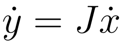
Where \(J\) is the Jacobian matrix and \(\dot{x}\) is the seed vector. For a detailed explanation of Jacobian-vector product see here.
Let’s implement a simple forward mode AD:
class Dual:
    def __init__(self, value, derivative):
        self.value = value
        self.derivative = derivative # works as \dot{x}

    def __add__(self, other):
        return Dual(self.value + other.value, self.derivative + other.derivative)

    def __mul__(self, other):
        return Dual(self.value * other.value,
                    self.value * other.derivative + self.derivative * other.value)

    def __pow__(self, n):
        return Dual(self.value ** n,
                    n * (self.value ** (n-1)) * self.derivative)
def f(x):
    return x**4 + 3*x**2 + 2*x

x = Dual(2.0, 1.0)  # x = 2, dx/dx = 1 (~> \dot{x})
result = f(x)

print(f"f(2) = {result.value}, f'(2) = {result.derivative}")
# >> Output: f(2) = 42.0, f'(2) = 58.0
As demonstrated, Forward autodiff augments each intermediate variable during evaluation of a function with its derivative. It involves replacing individual floating point values flowing through a function with tuples of the original intermediate values also called primals paired with their derivatives.
To compute the partial derivative of a function with respect to an input variable, we have to run a separate forward pass for each input variable of interest with corresponding seed set to 1. The forward mode autodiff produces one column of the corresponding Jacobian \(J\).
For a two dimensional input \(x \in \mathrm{R}^2\), setting \(\dot{x}\) to [1, 0] yields the first column of \(J\) which is the partial derivative w.r.t \(x_1\) and setting it to [0, 1] results in the second column which is the partial derivative w.r.t \(x_2\).
Ari Seff does a great job explaining it in his AutoDiff video here.
3.2 Reverse Mode
Reverse mode AutoDiff, which is the main AD method used in current major deep learning frameworks, computes gradients by propagating derivatives by going backward through the computation graph (see [6]) starting from the output and then applying the chain rule until it traverses the whole graph. It’s particularly efficient for functions with many inputs and few outputs, which is the typical case in neural networks [3].
Reverse mode computes the vector-Jacobian product which is explained PyTorch’s introduction to AtuoDiff in the “Vector Calculus using autograd” section here.
Here’s a simplified implementation of reverse mode AD:
class Node:
    def __init__(self, value):
        self.value = value
        self.grad = 0
        self._backward = lambda: None # this is defined as the forward mode is done based on the computation graph.
        self._prev = set()

    def __add__(self, other):
        other = other if isinstance(other, Node) else Node(other)
        out = Node(self.value + other.value)
        out._prev = {self, other}
        def _backward():
            self.grad += out.grad
            other.grad += out.grad
        out._backward = _backward
        return out

    def __mul__(self, other):
        other = other if isinstance(other, Node) else Node(other)
        out = Node(self.value * other.value)
        out._prev = {self, other}
        def _backward():
            self.grad += other.value * out.grad
            other.grad += self.value * out.grad
        out._backward = _backward
        return out

    def __pow__(self, n):
        out = Node(self.value ** n)
        out._prev = {self}

        def _backward():
            self.grad += n * (self.value ** (n-1)) * out.grad

        out._backward = _backward
        return out

def backward(node):
    topo = []
    visited = set()
    def build_topo(v):
        if v not in visited:
            visited.add(v)
            for child in v._prev:
                build_topo(child)
            topo.append(v)

    build_topo(node)
    node.grad = 1
    for node in reversed(topo):
        node._backward()


# Example usage
x = Node(2.0)

y = x**4 + 3*x**2 + 2*x

backward(y)

print(f"f(2) = {y.value}, f'(2) = {x.grad}")
# >> Output: f(2) = 42.0, f'(2) = 58.0
This implementation builds a computational graph and then traverses it backwards when the backward method is called on the output, to compute gradients, mimicking the process used in deep learning frameworks.
The key difference in computational complexity between forward and reverse modes becomes apparent when we consider functions with many inputs (parameters) and few outputs (typically a single loss value in ML), making reverse mode the preferred choice for deep learning [1]. the reason is that, in forward mode, computing the gradient for each input element \(x_i\) requires a separate forward pass through the computational graph.
4. Implementation Strategies: Operator Overloading vs. Source Transformation
4.1 Operator Overloading
Operator overloading, as demonstrated in our previous examples, redefines mathematical operations to compute both the result and its derivative. It’s the approach used by PyTorch and many Python-based AD libraries [4].
4.2 Source Transformation
Source transformation analyzes and modifies the source code to insert derivative computations. While more complex to implement, it can lead to more optimized code, especially for static computational graphs [1]. Tools like Tapenade use this approach.
Here’s a conceptual example of how source transformation might work:
# Original function
def f(x):
    return x**4 + 3*x**2 + 2*x

# Transformed function (conceptual, not actual code)
def f_and_gradient(x):
    # Forward pass
    t1 = x**2
    t2 = t1**2
    t3 = 3 * t1
    t4 = 2 * x
    y = t2 + t3 + t4

    # Backward pass
    dy = 1
    dt4 = dy
    dt3 = dy
    dt2 = dy
    dt1 = 2 * x * dt3 + 2 * t1 * dt2
    dx = 4 * x**3 * dy + 6 * x * dy + 2 * dy

    return y, dx
This transformed version computes both the function value and its gradient in a single pass through the code. As you can see, it is not as flexible and scalable for large-scale purposes such as in deep learning.
5. AutoDiff in the Wild: PyTorch vs. JAX
5.1 PyTorch
PyTorch uses a dynamic computational graph, built on-the-fly as operations are performed. This allows for flexibility in network architecture and easier debugging [5].
import torch

def f(x):
    return x**4 + 3*x**2 + 2*x

x = torch.tensor([2.0], requires_grad=True)
y = f(x)
y.backward()
print(f"f(2) = {y.item()}, f'(2) = {x.grad.item()}")
# Output: f(2) = 42.0, f'(2) = 58.0
PyTorch’s autograd engine records operations in a directed acyclic graph (DAG), where leaves are input tensors and roots are output tensors. During the backward pass, it computes gradients by traversing this graph [5].
For very detailed explanation to get a sense of how PyTorch’s autograd works, i would extremely recommend the first to videos of Andrej Karpathy’s Neural Networks: Zero to Hero playlist.
5.2 JAX
JAX, developed by Google Research, on the the hand uses a static computational graph and leverages XLA (Accelerated Linear Algebra) for efficient compilation to achieve better performance. It provides function transformations like grad for automatic differentiation, vmap for vectorization, and jit for compilation [4].
import jax
import jax.numpy as jnp

@jax.jit
def f(x):
    return x**4 + 3*x**2 + 2*x

df = jax.grad(f)

x = 2.0
print(f"f(2) = {f(x)}, f'(2) = {df(x)}")
# Output: f(2) = 42.0, f'(2) = 58.0

# Vectorized computation
vdf = jax.vmap(df)
x_vec = jnp.array([1.0, 2.0, 3.0])

print(f"f'(x) for x=[1,2,3]: {vdf(x_vec)}")
# Output: f'(x) for x=[1,2,3]: [10. 58. 154.]
JAX’s approach allows for efficient compilation and execution on accelerators like GPUs and TPUs [4]. Check out the “The Autodiff Cookbook” from JAX developers for a more technical grasp of their implementations.
Note the difference that PyTorch’s implementation requires that first a forward pass is done with an input, then as the backwards are computed, the gradients are accessible, whereas in JAX, the jax.grad transformation can be called on any defined function without the need to calling the function itself manually.
6. Some Advanced Topics in AutoDiff
6.1 Higher-Order Derivatives
One thing o note is that AutoDiff isn’t limited to first-order derivatives. By applying AD to its own output, we can compute higher-order derivatives. This is crucial for optimization algorithms like Newton’s method that use second-order information (Hessians).
In JAX particularly, computing higher-order derivatives is pretty straightforward:
import jax
import jax.numpy as jnp


def f(x):
    return x**4 + 3*x**2 + 2*x

ddf = jax.grad(jax.grad(f))
x = 2.0

print(f"f''(2) = {ddf(x)}")
# Output: f''(2) = 102.0
just call the grad function transformation twice on your function and you’re good to go.
6.2 Vector-Jacobian Products (VJPs) and Jacobian-Vector Products (JVPs)
VJPs and JVPs are the building blocks of reverse and forward mode AD, respectively. Understanding these operations is crucial for implementing efficient custom gradients.
JAX provides explicit functions for these operations:
import jax
import jax.numpy as jnp


def f(x):
    return jnp.array([x**2, x**3])

x = 2.0
y, vjp_fn = jax.vjp(f, x)

print(f"VJP: {vjp_fn(jnp.array([1.0, 1.0]))[0]}")

primal, jvp_fn = jax.jvp(f, (x,), (1.0,))
print(f"JVP: {jvp_fn}")

# Output:
# VJP: 16.0
# JVP: [4. 12.]
6.3 AD through Iterative Processes
Applying AD to iterative processes like optimization loops or recurrent neural networks requires careful handling to avoid excessive memory usage. Techniques like checkpointing and reversible computations are used to balance memory usage and computational cost [1].
7. The Impact of AutoDiff on Deep Learning
AutoDiff, particularly reverse mode AD, has been instrumental in the deep learning revolution. It allows efficient computation of gradients for millions of parameters with respect to a loss value. This efficiency enables the training of increasingly complex models, driving advancements in areas like natural language processing, computer vision, and reinforcement learning [2].
Some key impacts to mention:
-
Architectural Flexibility: AD allows researchers to easily experiment with novel network architectures without manually deriving gradients.
-
Computational Efficiency: Reverse mode AD makes it feasible to train very deep networks with millions or billions of parameters.
-
Higher-Order Optimization: Easy access to higher-order derivatives enables more sophisticated optimization techniques.
-
Custom Differentiable Operations: Researchers can define custom differentiable operations, expanding the range of possible model architectures.
8. Conclusion and Future Directions
Automatic Differentiation has become an indispensable tool in machine learning, enabling the training of increasingly complex models. As we push the boundaries of AI, several exciting directions for AD research emerge:
-
AD for Probabilistic Programming: Extending AD to handle probabilistic computations and enable more flexible Bayesian inference.
-
Differentiable Programming: Moving beyond traditional neural networks to make entire programs differentiable.
-
Hardware-Specific Optimizations: Tailoring AD algorithms for specialized AI hardware.
-
AD for Sparse and Structured Computations: Developing efficient AD techniques for sparse or structured problems common in scientific computing.
As these areas develop, we can expect AutoDiff to continue playing a crucial role in advancing the field of machine learning and artificial intelligence.
References
[1] Baydin, A. G., Pearlmutter, B. A., Radul, A. A., & Siskind, J. M. (2018). Automatic differentiation in machine learning: a survey. Journal of Machine Learning Research, 18, 1–43.
[2] Grosse, R. (2019). Automatic Differentiation. CSC421/2516 Lecture Notes, University of Toronto.
[3] Andmholm. (2023). What is Automatic Differentiation. Hugging Face Blog.
[4] JAX Team. (2024). Automatic Differentiation and the JAX Ecosystem. JAX Documentation.
[5] PyTorch Team. (2024). Autograd: Automatic Differentiation. PyTorch Tutorials.